


Local Floo hazard - Urban scale
For river reaches containing backwater areas, naturally occurring diversion channels and inundation areas at local scale, the 1D assumptions are frequently violated. For out-of-bank flow, interaction with the floodplain results in highly complex fluid movement with at least two-dimensional properties, which can be computationally affordable for medium size domains. Local flood hazard mapping allows for evaluating water depth and velocity and, at the urban scale, the most sensitive working assumption is the representation of buildings.
The complex interaction of channel and floodplain flow fields make two-dimensional simulation codes more desirable than one-dimensional codes in many modeling situations (Cunge 1969; Horritt & Bates 2002). Continual improvements in computational resources and affordability have also increased implementation of two-dimensional modeling. Most widely used two-dimensional codes utilize depth-averaged Navier-Stokes equations, commonly called the Saint-Venant Shallow Water Equations (SWE):
![]() (1)
(1)
where U is the variables vector, F and Fd and G and Gd are the convective and diffusive fluxes vectors in the x and y directions respectively (in the plane of movement). H is the friction and slope source term vector and I the infiltration source vector. The expressions for vectors U, F, G above read:
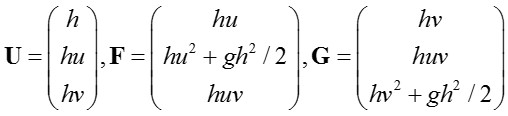 (2)
(2)
where h is water depth, u and v are the averaged (over the depth and time in a turbulent flow) cartesian velocity components, and g the acceleration of gravity. The corresponding expressions for the diffusive fluxes Fd, Gd can be written:
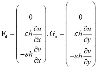 (3)
(3)
Where ε is a kinematic viscosity coefficient that accounts for the fluid kinematic viscosity, the turbulent eddy viscosity and the apparent viscosity due to the velocity fluctuations about the vertical average. Finally H and I read:
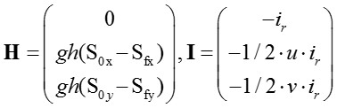 (4)
(4)
Here iris the infiltration rate into the ground/sinks, S0x and S0y are the bed slopes in the two Cartesian directions, which are assumed small:
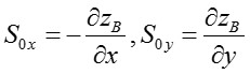 (5)
(5)
where zB is the bottom surface and Sfx, Sfy are the friction slopes, usually represented by means of an empirical formula, in this case Manning’s:
![]() (6)
(6)
Where n is the Manning’s friction coefficient.
However, the shallow water equations are not a true mathematical representation of the movement of water over the earth surface (Alcrudo, 2004). Putting aside errors originated from a numerical integration of these equations, the following known shortcomings of this approximation stand:
- • Vertical velocities are neglected (vertical acceleration are identically zero)
- • The pressure field is assumed hydrostatic
- • The bottom slope is assumed small
- • A uniform horizontal velocity field is assumed across the water layer
- • Turbulence effects are usually ignored
- • Friction formulae are usually taken from uniform flow conditions
The use of 2D equations enables to choose different levels of approximation with increasing complexity, the kinematic, the diffusive and the full dynamic wave (Hunter et al. 2007).
Kinematic wave can be described by a simple partial differential equation with a single unknown field variable (e.g., the flow or wave height) in terms of the two independent variables the time (t) and the space (x) with some parameters containing information about the physics and geometry of the flow. This approximation is usually adopted in upstream and midstream steep channel reaches to avoid numerical instability when performing a flood forecast. When these assumptions can’t be made, the diffusive wave approximation is considered as adequate for flood simulations (Hunter et al. 2008).
The SWE system being of hyperbolic character in time it represents an evolutionary problem in the form of propagating waves. Therefore a time marching procedure starting with a given initial condition in space, supplemented with boundary conditions along the time path is the proper mathematical conceptual treatment. The discretization of SWE can be made with different approaches: Finite Elements, Finite Volume and Finite Difference (Ferziger, J.H., Peric 2002).
2D models require as geometry data the bathymetry of the study area in order to generate a computational mesh of the domain. The resolution of the computational mesh varies, according to the scale of analysis, between 1 m (for dense urban areas) and 500-1000 m for macro-scale studies (e.g. at a national or regional level) (Falter et al. 2013; Syme 2008; Hunter et al. 2008).
The sustainable complexity of a model depends on the amount of available data and computational resources. Flood propagation in urban areas is clearly two-dimensional, with peculiar features that depend on the complex interaction between the flow and the streets/buildings pattern, especially when the urban texture is very dense as in many historic town centres (Arrighi et al. 2013).
One of the challenges for the modeller for local scale flood hazard analysis is how best to represent the roads, fences, houses and other features within the limitations and constraints to work with. 2D solutions are very computationally intensive and it is not always practical to utilise a mesh of very fine elements. This forces to make approximations when representing the urban domain to represent the fences, buildings, and other obstructions.
In some cases 1D numerical models are considered as adequate for the estimation of flood-water levels in river with regular flow patterns and the preliminary identification of inundation zones (Apel et al. 2009; Messner et al. 2007). When there are more complex river geometries and inundation flow patterns are relevant for the precise mapping of local parameters, the use of 2D model becomes unavoidable (Galland et al. 1991; Hervouet et al. 2000; Büchele et al. 2006; Apel et al. 2009; Ernst et al. 2010). Diffusive full 2D models are potentially more accurate than 1D or quasi-2D models, but they are more difficult to apply systematically to large areas if only traditional elevation data are available. They require two crucial pieces of information to achieve their potential accuracy: the detailed topography of the flow domain, including buildings and infrastructures, and its representative roughness.
LIDAR-based aerial survey generates high quality topographic data and enables to obtain a complete, high resolution (e.g. order of 1 m nominal spacing or even less) and up-to-date Digital Surface Model (DSM). Recently this kind of products has become increasingly available also in dense urban areas, so with this respect the problem is no more in the data availability, it is rather in the computational difficulties, resolution and structure of the computational grid, related to the streets/buildings pattern. The determination of roughness coefficients also needs an accurate and high resolution land use database, to be eventually augmented with the increase of friction due to irregular topography (Ernst et al. 2010; Syme 2008). The advantages of a ‘classical’ 2D model over a more parsimonious one can be strongly reduced if other simplifications are required for their practical implementation, such as a steady-state approximation (Ernst et al. 2010) or an upper bound to the computational nodes. 2D hydraulic models have usually been adopted in portions of sparse urban areas, providing reliable results after calibration studies (Apel et al. 2009; Ernst et al. 2010; de Moel et al. 2009; Schubert & Sanders 2012; Ma et al. 2015). For such a study in a dense urban environment some problems arise in the set-up of a 2D model. First of all the computational costs which is recognized as the major drawback of 2D models performed with a fine grid size (Begnudelli et al. 2008; Chen et al. 2012). A grid size of 1 or 2 m is generally considered as unavoidable to describe the street pattern of many urban environments, especially when historic centres are included, and may lead to long simulations.
The combination of a 1D model for the main river channel flow and a 2D model for the inundated areas is recognized as a good compromise between complexity and accuracy. Shallow water equations or their diffusive wave approximation are theoretically optimal choices for the 2D part, but the use of storage cells (Bates & De Roo 2000; Huang et al. 2007; Horritt & Bates 2002) has been also proposed when the above difficulties arise.